传感器简介

移动机器人装备了大量的传感器，因此它们能够看见和感知周围的环境。这些传感器获取的信息被用于构建和维护环境地图、在地图上定位机器人以及观察环境中的障碍物。这些任务对于在动态环境中安全而有效地导航机器人至关重要。

常用的传感器有lidar，radar，RGB camera，depth camera，IMU和GPS。为了统一这些传感器的消息格式以便传感器供应商之间更容易合作，ROS提供了sensor_msgs功能包来定义通用的传感器接口。这使得用户可以使用任意供应商的产品，只要它遵循了sensor_msgs的标准格式。

目前导航中常用的消息格式有：sensor_msgs/LaserScan，sensor_msgs/PointCloud2，sensor_mgs/Range，sensor_mgs/Image。此外，radar_msgs限用于特定的雷达传感器，vision_msgs功能包则定义了机器视觉中使用的消息，如故障检测、分割以及其他机器学习模型。举几个例子，vision_msgs/Classification2D，vision_msgs/Classification3D，vision_msgs/Detection2D，和vision_msgs/Detection3D。

更多信息可以参考，sensor_msgs, radar_msgs, and vision_msgs.

对于一个真实的物理机器人，它的传感器可能已经拥有了ROS驱动程序（以node节点的形式，连接到传感器上，将传感器数据填写到消息中，然后发布供机器人使用），这些驱动程序遵循sensor_msgs中的标准接口。sensor_msgs功能包让我们能轻松使用不同供应商的传感器。

对于仿真的机器人，Gazebo提供了传感器插件来发布符合sensor_msgs标准的消息。

常见的传感器消息类型

sensor_msgs/LaserScan

它来自平面激光的单次扫描，它被slam_toolbox和nav2_amcl功能包所使用，来完成定位和建图的任务，也可以被nav2_costmap_2d功能包用于感知任务。

../../_images/sensor_laserscan.png

sensor_msgs/PointCloud2

这个消息持有了一个3D点的集合，以及关于每个点的可选附加信息。它的来源可以是3D lidar，2D lidar，深度相机或者其设备。

../../_images/sensor_pointcloud2.png

sensor_msgs/Range

它是一个来自活跃测距仪的单一距离读数，测距仪发出能量射线，随后报告一个沿着弧线测量距离的有效读数。如声呐、红外传感器或一维测距仪。

../../_images/sensor_range.png

sensor_msgs/Image

它表示来自RGB或者深度相机的传感器读数，对应于RGB值或者范围值

../../_images/sensor_image.png

使用Gazebo模拟传感器

类似于上一篇文章中用Gazebo插件添加里程计到机器人sam_bot上，我们同样将使用Gazebo插件去模拟一个lidar(激光雷达)和一个深度相机。

即便我们是在使用一个真实的机器人，这里的大多数步骤对于建立URDF框架依然是必需的，添加Gazebo插件不会引入任何问题。

向URDF文件添加Gazebo插件

添加lidar到sam_bot，打开文件sam_bot_description.urdf，在标签之前插入以下内容

<link name="lidar_link">
  <inertial>
    <origin xyz="0 0 0" rpy="0 0 0"/>
    <mass value="0.125"/>
    <inertia ixx="0.001"  ixy="0"  ixz="0" iyy="0.001" iyz="0" izz="0.001" />
  </inertial>

  <collision>
    <origin xyz="0 0 0" rpy="0 0 0"/>
    <geometry>
       <cylinder radius="0.0508" length="0.055"/>
    </geometry>
  </collision>

  <visual>
    <origin xyz="0 0 0" rpy="0 0 0"/>
    <geometry>
       <cylinder radius="0.0508" length="0.055"/>
    </geometry>
  </visual>
</link>

<joint name="lidar_joint" type="fixed">
  <parent link="base_link"/>
  <child link="lidar_link"/>
  <origin xyz="0 0 0.12" rpy="0 0 0"/>
</joint>

<gazebo reference="lidar_link">
  <sensor name="lidar" type="ray">
    <always_on>true</always_on>
    <visualize>true</visualize>
    <update_rate>5</update_rate>
    <ray>
      <scan>
        <horizontal>
          <samples>360</samples>
          <resolution>1.000000</resolution>
          <min_angle>0.000000</min_angle>
          <max_angle>6.280000</max_angle>
        </horizontal>
      </scan>
      <range>
        <min>0.120000</min>
        <max>3.5</max>
        <resolution>0.015000</resolution>
      </range>
      <noise>
        <type>gaussian</type>
        <mean>0.0</mean>
        <stddev>0.01</stddev>
      </noise>
    </ray>
    <plugin name="scan" filename="libgazebo_ros_ray_sensor.so">
      <ros>
        <remapping>~/out:=scan</remapping>
      </ros>
      <output_type>sensor_msgs/LaserScan</output_type>
      <frame_name>lidar_link</frame_name>
    </plugin>
  </sensor>
</gazebo>

在这段代码中，我们创建了一个lidar_link，它被gazebo_ros_ray_sensor插件引用为添加传感器的位置。我们还设置了模拟的lidar扫描和范围属性，/scan作为发送sensor_msgs/LaserScan消息的话题。

添加深度相机到sam_bot，在上一段的标签后插入以下内容

<link name="camera_link">
  <visual>
    <origin xyz="0 0 0" rpy="0 0 0"/>
    <geometry>
      <box size="0.015 0.130 0.022"/>
    </geometry>
  </visual>

  <collision>
    <origin xyz="0 0 0" rpy="0 0 0"/>
    <geometry>
      <box size="0.015 0.130 0.022"/>
    </geometry>
  </collision>

  <inertial>
    <origin xyz="0 0 0" rpy="0 0 0"/>
    <mass value="0.035"/>
    <inertia ixx="0.001"  ixy="0"  ixz="0" iyy="0.001" iyz="0" izz="0.001" />
  </inertial>
</link>

<joint name="camera_joint" type="fixed">
  <parent link="base_link"/>
  <child link="camera_link"/>
  <origin xyz="0.215 0 0.05" rpy="0 0 0"/>
</joint>

<link name="camera_depth_frame"/>

<joint name="camera_depth_joint" type="fixed">
  <origin xyz="0 0 0" rpy="${-pi/2} 0 ${-pi}"/>
  <parent link="camera_link"/>
  <child link="camera_depth_frame"/>
</joint>

<gazebo reference="camera_link">
  <sensor name="depth_camera" type="depth">
    <visualize>true</visualize>
    <update_rate>30.0</update_rate>
    <camera name="camera">
      <horizontal_fov>1.047198</horizontal_fov>
      <image>
        <width>640</width>
        <height>480</height>
        <format>R8G8B8</format>
      </image>
      <clip>
        <near>0.05</near>
        <far>3</far>
      </clip>
    </camera>
    <plugin name="depth_camera_controller" filename="libgazebo_ros_camera.so">
      <baseline>0.2</baseline>
      <alwaysOn>true</alwaysOn>
      <updateRate>0.0</updateRate>
      <frameName>camera_depth_frame</frameName>
      <pointCloudCutoff>0.5</pointCloudCutoff>
      <pointCloudCutoffMax>3.0</pointCloudCutoffMax>
      <distortionK1>0</distortionK1>
      <distortionK2>0</distortionK2>
      <distortionK3>0</distortionK3>
      <distortionT1>0</distortionT1>
      <distortionT2>0</distortionT2>
      <CxPrime>0</CxPrime>
      <Cx>0</Cx>
      <Cy>0</Cy>
      <focalLength>0</focalLength>
      <hackBaseline>0</hackBaseline>
    </plugin>
  </sensor>
</gazebo>

同样，我们创建了一个camera_link，它被gazebo_ros_camera插件引用来作为添加传感器的位置。我们还创建了一个camera_depth_frame依附于camera_link上，它被设置为深度相机插件的。我们为这个插件设置了话题/depth_camera/image_raw和/depth_camera/points来发布sensor_msgs/Image和sensor_msgs/PointCloud2两个消息。最后我们做了一些其他的基本配置。

编译与运行

为了验证传感器能正常运作，我们需要在一个Gazebo的仿真世界里启动sam_bot。

创建一个带圆柱体与球体的Gazebo世界

在工程根目录下创建world目录，在目录中新建文件my_world.sdf，插入以下内容

<sdf version='1.7'>
  <world name='default'>
    <light name='sun' type='directional'>
      <cast_shadows>1</cast_shadows>
      <pose>0 0 10 0 -0 0</pose>
      <diffuse>0.8 0.8 0.8 1</diffuse>
      <specular>0.2 0.2 0.2 1</specular>
      <attenuation>
        <range>1000</range>
        <constant>0.9</constant>
        <linear>0.01</linear>
        <quadratic>0.001</quadratic>
      </attenuation>
      <direction>-0.5 0.1 -0.9</direction>
      <spot>
        <inner_angle>0</inner_angle>
        <outer_angle>0</outer_angle>
        <falloff>0</falloff>
      </spot>
    </light>
    <model name='ground_plane'>
      <static>1</static>
      <link name='link'>
        <collision name='collision'>
          <geometry>
            <plane>
              <normal>0 0 1</normal>
              <size>100 100</size>
            </plane>
          </geometry>
          <surface>
            <friction>
              <ode>
                <mu>100</mu>
                <mu2>50</mu2>
              </ode>
              <torsional>
                <ode/>
              </torsional>
            </friction>
            <contact>
              <ode/>
            </contact>
            <bounce/>
          </surface>
          <max_contacts>10</max_contacts>
        </collision>
        <visual name='visual'>
          <cast_shadows>0</cast_shadows>
          <geometry>
            <plane>
              <normal>0 0 1</normal>
              <size>100 100</size>
            </plane>
          </geometry>
          <material>
            <script>
              <uri>file://media/materials/scripts/gazebo.material</uri>
              <name>Gazebo/Grey</name>
            </script>
          </material>
        </visual>
        <self_collide>0</self_collide>
        <enable_wind>0</enable_wind>
        <kinematic>0</kinematic>
      </link>
    </model>
    <gravity>0 0 -9.8</gravity>
    <magnetic_field>6e-06 2.3e-05 -4.2e-05</magnetic_field>
    <atmosphere type='adiabatic'/>
    <physics type='ode'>
      <max_step_size>0.001</max_step_size>
      <real_time_factor>1</real_time_factor>
      <real_time_update_rate>1000</real_time_update_rate>
    </physics>
    <scene>
      <ambient>0.4 0.4 0.4 1</ambient>
      <background>0.7 0.7 0.7 1</background>
      <shadows>1</shadows>
    </scene>
    <wind/>
    <spherical_coordinates>
      <surface_model>EARTH_WGS84</surface_model>
      <latitude_deg>0</latitude_deg>
      <longitude_deg>0</longitude_deg>
      <elevation>0</elevation>
      <heading_deg>0</heading_deg>
    </spherical_coordinates>
    <model name='unit_box'>
      <pose>1.51271 -0.181418 0.5 0 -0 0</pose>
      <link name='link'>
        <inertial>
          <mass>1</mass>
          <inertia>
            <ixx>0.166667</ixx>
            <ixy>0</ixy>
            <ixz>0</ixz>
            <iyy>0.166667</iyy>
            <iyz>0</iyz>
            <izz>0.166667</izz>
          </inertia>
          <pose>0 0 0 0 -0 0</pose>
        </inertial>
        <collision name='collision'>
          <geometry>
            <box>
              <size>1 1 1</size>
            </box>
          </geometry>
          <max_contacts>10</max_contacts>
          <surface>
            <contact>
              <ode/>
            </contact>
            <bounce/>
            <friction>
              <torsional>
                <ode/>
              </torsional>
              <ode/>
            </friction>
          </surface>
        </collision>
        <visual name='visual'>
          <geometry>
            <box>
              <size>1 1 1</size>
            </box>
          </geometry>
          <material>
            <script>
              <name>Gazebo/Grey</name>
              <uri>file://media/materials/scripts/gazebo.material</uri>
            </script>
          </material>
        </visual>
        <self_collide>0</self_collide>
        <enable_wind>0</enable_wind>
        <kinematic>0</kinematic>
      </link>
    </model>
    <model name='unit_sphere'>
      <pose>-1.89496 2.36764 0.5 0 -0 0</pose>
      <link name='link'>
        <inertial>
          <mass>1</mass>
          <inertia>
            <ixx>0.1</ixx>
            <ixy>0</ixy>
            <ixz>0</ixz>
            <iyy>0.1</iyy>
            <iyz>0</iyz>
            <izz>0.1</izz>
          </inertia>
          <pose>0 0 0 0 -0 0</pose>
        </inertial>
        <collision name='collision'>
          <geometry>
            <sphere>
              <radius>0.5</radius>
            </sphere>
          </geometry>
          <max_contacts>10</max_contacts>
          <surface>
            <contact>
              <ode/>
            </contact>
            <bounce/>
            <friction>
              <torsional>
                <ode/>
              </torsional>
              <ode/>
            </friction>
          </surface>
        </collision>
        <visual name='visual'>
          <geometry>
            <sphere>
              <radius>0.5</radius>
            </sphere>
          </geometry>
          <material>
            <script>
              <name>Gazebo/Grey</name>
              <uri>file://media/materials/scripts/gazebo.material</uri>
            </script>
          </material>
        </visual>
        <self_collide>0</self_collide>
        <enable_wind>0</enable_wind>
        <kinematic>0</kinematic>
      </link>
    </model>
    <state world_name='default'>
      <sim_time>0 0</sim_time>
      <real_time>0 0</real_time>
      <wall_time>1626668720 808592627</wall_time>
      <iterations>0</iterations>
      <model name='ground_plane'>
        <pose>0 0 0 0 -0 0</pose>
        <scale>1 1 1</scale>
        <link name='link'>
          <pose>0 0 0 0 -0 0</pose>
          <velocity>0 0 0 0 -0 0</velocity>
          <acceleration>0 0 0 0 -0 0</acceleration>
          <wrench>0 0 0 0 -0 0</wrench>
        </link>
      </model>
      <model name='unit_box'>
        <pose>1.51272 -0.181418 0.499995 0 1e-05 0</pose>
        <scale>1 1 1</scale>
        <link name='link'>
          <pose>1.51272 -0.181418 0.499995 0 1e-05 0</pose>
          <velocity>0 0 0 0 -0 0</velocity>
          <acceleration>0.010615 -0.006191 -9.78231 0.012424 0.021225 1.8e-05</acceleration>
          <wrench>0.010615 -0.006191 -9.78231 0 -0 0</wrench>
        </link>
      </model>
      <model name='unit_sphere'>
        <pose>-0.725833 1.36206 0.5 0 -0 0</pose>
        <scale>1 1 1</scale>
        <link name='link'>
          <pose>-0.944955 1.09802 0.5 0 -0 0</pose>
          <velocity>0 0 0 0 -0 0</velocity>
          <acceleration>0 0 0 0 -0 0</acceleration>
          <wrench>0 0 0 0 -0 0</wrench>
        </link>
      </model>
      <light name='sun'>
        <pose>0 0 10 0 -0 0</pose>
      </light>
    </state>
    <gui fullscreen='0'>
      <camera name='user_camera'>
        <pose>3.17226 -5.10401 6.58845 0 0.739643 2.19219</pose>
        <view_controller>orbit</view_controller>
        <projection_type>perspective</projection_type>
      </camera>
    </gui>
  </world>
</sdf>

修改launch文件display.launch.py

添加my_world.sdf的路径到generate_launch_description():

1	world_path=os.path.join(pkg_share, 'world/my_world.sdf'),

同样需要添加world的路径到以下位置

1	launch.actions.ExecuteProcess(cmd=['gazebo', '--verbose', '-s', 'libgazebo_ros_factory.so', world_path], output='screen'),

修改CMakeLists

install(
  DIRECTORY src launch rviz config world
  DESTINATION share/${PROJECT_NAME}
)

编译并运行

1
2
3

colcon build
. install/setup.bash
ros2 launch sam_bot_description display.launch.py

在rviz中显示sensor_msgs/LaserScan消息

在LaserScan列表中展开topic，将Reliability Policy设置为Best Effort，size设置为0.1以便更清晰的观察点云。

![](/home/ubuntu-ros2/myBlog/source/_posts/Navigation2专题五：设置传感器/Peek 2021-08-18 18-09.gif)

为了可视化sensor_msgs/Image消息和sensor_msgs/PointCloud2消息，可以参照LaserScan操作

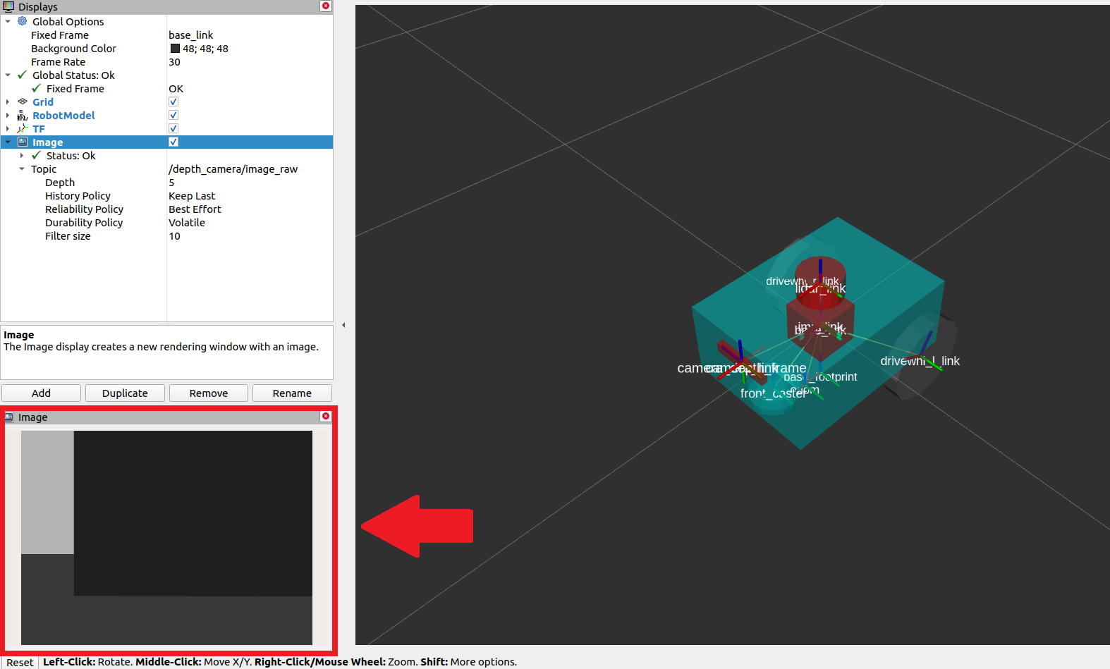
上图为官方结果，实际结果添加image话题后，看不到图像

需要将Reliability Policy设置为Best Effort

下方为PointCloud2的结果

建图与定位

slam_toolbox是一个具备2D SLAM能力的ROS2工具集，也是Nav2官方支持的SLAM库之一。当你需要在机器人中配置SLAM时，官方推荐使用slam_toolbox工具集。此外nav2_amcl功能包也可以实现定位，它使用自适应蒙特卡洛方法（Adaptive Monte Carlo Localization）去估计机器人在地图中的位姿和方向。

slam_toolbox与nav2_amcl都采用激光扫描信息去感知机器人周边的环境。因此，为了验证它们是否可以访问激光扫描传感器的读数，我们必须确保它们都订阅了sensor_msgs/LaserScan对应的正确话题。这个可以通过设置它们的scan_topic参数来实现。目前sensor_msgs/LaserScan消息发送到/scan话题中是一种默认的约定，因此，scan_topic要被设置为/scan。

如果需要更深入的了解完整的参数配置过程，请参考Github repository of slam_toolbox与AMCL Configuration Guide。

Costmap 2D

costmap 以占用网格（occupancy grid）的形式使用传感器信息来描述机器人周边的环境。占用网格的单元格存储着0-254区间内的代价值，表示机器人穿过这些区域的代价。0代价表示单元格空闲，而254则表示单元格被完全占据。导航算法使用这两个极端情况之间的数值去引导机器人远离障碍。Nav2中的代价地图是由功能包nav2_costmap_2d实现的。
costmap分层
- static layer：表示代价地图的地图部分，它捕获发布到/map话题上的消息（比如由SLAM产生的）来构建这个部分。
- obstacle layer：体现的是由传感器检测到的物体（比如障碍物），这些传感器在探测过程中会发布LaserScan或者PointCloud2消息，也同时可以发布他们两个消息。
- voxel layer：类似于obstacle layer，但它处理3D数据。
- range layer：体现的是由声呐和红外传感器检测到的信息。
- inflation layer：表示环绕致命障碍物的附加代价，用于帮助机器人躲避由于它的几何形状引发的碰撞。如果膨胀层被启用，那么需要用户指定一个膨胀半径。

更多的内容可以参考ROS1 costmap_2D documentation

配置nav2_costmap_2d

以sam_bot的lidar传感器为例，配置nav2_costmap_2d。我们将展示static layer, obstacle layer, voxel layer和inflation layer的配置。我们令obstacle和voxel层都使用LaserScan消息。我们还将设置一些基本参数用于定义如何把障碍物映射到代价地图中。

下方这些配置信息被包含在Nav2的配置文件中

global_costmap:
  global_costmap:
    ros__parameters:
      update_frequency: 1.0
      publish_frequency: 1.0
      global_frame: map
      robot_base_frame: base_link
      use_sim_time: True
      robot_radius: 0.22
      resolution: 0.05
      track_unknown_space: false
      rolling_window: false
      plugins: ["static_layer", "obstacle_layer", "inflation_layer"]
      static_layer:
        plugin: "nav2_costmap_2d::StaticLayer"
        map_subscribe_transient_local: True
      obstacle_layer:
        plugin: "nav2_costmap_2d::ObstacleLayer"
        enabled: True
        observation_sources: scan
        scan:
          topic: /scan
          max_obstacle_height: 2.0
          clearing: True
          marking: True
          data_type: "LaserScan"
          raytrace_max_range: 3.0
          raytrace_min_range: 0.0
          obstacle_max_range: 2.5
          obstacle_min_range: 0.0
      inflation_layer:
        plugin: "nav2_costmap_2d::InflationLayer"
        cost_scaling_factor: 3.0
        inflation_radius: 0.55
      always_send_full_costmap: True

local_costmap:
  local_costmap:
    ros__parameters:
      update_frequency: 5.0
      publish_frequency: 2.0
      global_frame: odom
      robot_base_frame: base_link
      use_sim_time: True
      rolling_window: true
      width: 3
      height: 3
      resolution: 0.05
      robot_radius: 0.22
      plugins: ["voxel_layer", "inflation_layer"]
      voxel_layer:
        plugin: "nav2_costmap_2d::VoxelLayer"
        enabled: True
        publish_voxel_map: True
        origin_z: 0.0
        z_resolution: 0.05
        z_voxels: 16
        max_obstacle_height: 2.0
        mark_threshold: 0
        observation_sources: scan
        scan:
          topic: /scan
          max_obstacle_height: 2.0
          clearing: True
          marking: True
          data_type: "LaserScan"
      inflation_layer:
        plugin: "nav2_costmap_2d::InflationLayer"
        cost_scaling_factor: 3.0
        inflation_radius: 0.55
      always_send_full_costmap: True

global_costmap：主要用于整个地图的长周期规划。
local_costmap：用于短周期规划与避障。
我们需要配置的图层需要在plugins参数中配置，如global_costmap中的13行（plugins: 这行）以及local_costmap中的50行。这些图层名以列表的形式存储，他们也是之后每一个图层参数的命名空间。每一个图层都需要一个plugin参数用于定义为其对应的插件类型。
static layer：map_subsrcribe_transient_local参数为True，它设置的是map话题的Qos。而map_topic这是设置了订阅的map话题名，如果没有写则默认为/map。
obstacle layer：首先定义了传感器源observation_sources参数为scan，之后便是传感器源本身的参数。topic参数是传感器发布的话题名，data_type参数则是话题对应的消息类型，这里分别是/scan与LaserScan。其他参数，max_obstacle_height用于设置返回给占用网格的传感器读数的最大高度，min_obstacle_height则是最小高度（如果不配置默认为0）。clearing参数用于设置是否将障碍物从代价地图中移除。清除操作通过穿越网格的射线追踪来完成。我们使用raytrace_max_range和raytrace_min_range两个参数来设置从代价地图清除障碍物的范围。marking参数用于设置被插入的障碍物是否在代价地图上标记出来。obstacle_max_range和obstacle_min_range用于设置在代价地图中标记障碍物的方位。

voxel layer：与obstacle layer相似，如果向同时使用LaserScan和PointCloud2作为传感器源，需要做如下调整

obstacle_layer:
  plugin: "nav2_costmap_2d::ObstacleLayer"
  enabled: True
  observation_sources: scan pointcloud
  scan:
    topic: /scan
    data_type: "LaserScan"
  pointcloud:
    topic: /depth_camera/points
    data_type: "PointCloud2"

publish_voxel_map设置为True以使能3D网格的发布。z_resolution高度上的分辨率，而每列中voxel的数量则是用z_voxels定义。mark_threshold设置每一列中voxel的最小数量来作为占用网格中被占用的标记。observation_sources与obstacle layer类似。

inflation layer：cost_scaling_factor参数设置了膨胀半径的指数衰减因子。inflation_radius定义了障碍物的膨胀半径。
我们没有使用range layer，但它或许对于其他机器人也是有用的。它的基本参数topics（订阅的话题列表）， input_sensor_type（可以是ALL，VARIABLE或者FIXED）和clear_on_max_reading（bool类型，决定是否在最大距离清除传感器读数）。

更多内容可以参考 Costmap 2D Configuration Guide

编译运行与验证

首先启动display.launch.py，他会运行robot state Publisher提供base_link=>sensors的坐标变化；运行Gazebo作为物理仿真器并提供odom=>base_link的坐标变化（通过差速驱动插件）；运行rviz完成机器人和传感器信息的可视化。
1
2
3
colcon build
. install/setup.bash
ros2 launch sam_bot_description display.launch.py
接着，启动slam_toolbox 去发布/map话题并提供map=>odom的变换。/map话题将被global_costmap的static layer使用。
1
sudo apt install ros-<ros2-distro>-slam-toolbox
安装rolling版本的slam_toolbox，可惜rolling没有实现slam_toolbox，建议使用foxy或者galactic
1
ros2 launch slam_toolbox online_async_launch.py
此时slam_toolbox已经开始发布/map话题并提供map=>odom的变换。

我们在rviz中添加/map话题，就能看到下面的可视化消息
启动Nav2系统。目前我们值会探索Nav2的代价地图生成系统。在启动Nav2后，我们将在rviz中可视化代价地图。
检查变换是否正确，执行以下命令
1
ros2 run tf2_tools view_frames.py
事实上，执行的命令为
1
ros2 run tf2_tools view_frames
实际效果为

启动Nav2

确保Nav2已经安装

1 2	sudo apt install ros-<ros2-distro>-navigation2 sudo apt install ros-<ros2-distro>-nav2-bringup

启动Nav2
1
ros2 launch nav2_bringup navigation_launch.py
之前我们讨论过的nav2_costmap_2d的参数都包含在navigation_launch.py的默认参数中。此外，该文件中还包含Nav2应用中其他节点的参数。

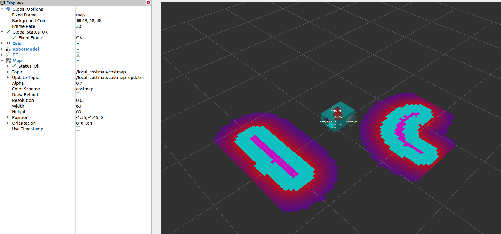
在rviz中可视化Costmaps

global_costmap，local_costmap和检测到的障碍物的体素（体积元素voxel）都可以在rivz中可视化。

可视化global_costmap，需要在rviz中选择/global_costmap/costmap话题下的Map
可视化local_costmap，选择/local_costmap/costmap下的Map
可视化障碍物的体素（voxel），输入命令
1
ros2 run nav2_costmap_2d nav2_costmap_2d_markers voxel_grid:=/local_costmap/voxel_grid visualization_marker:=/my_marker
在rviz中选择/my_marker话题下的Marker

然后将fixed frame设置为odom，

Navigation2专题五：设置传感器

传感器简介

常见的传感器消息类型

使用Gazebo模拟传感器

建图与定位

Tags

FRIENDS